The future will soon be a thing of past
Blogpost will talk about need and what of Autoregressive models, but before going towards the what, its’ better to first understand why we felt the need to have another type of models in machine learning community. We will look at the Motivation behind the creation and what problems we want to solve using them.
Motivation
Problems we would like to solve
- Generating Data: syntheizing images, text, videos, speech
- Compressing data: constructing efficient codes.
- Anomaly Detection: e.g. supervised estimator is forced to make a decision even over the datapoint it is uncertain about
Suppose there exist true data distribution \(p_{data}(\textbf{x})\), now you most probably will not be able to know this distribution but what you can do is sample some data points from it \(\textbf{x}^{(1)}, \textbf{x}^{(2)} … \textbf{x}^{(n)} \sim p_{data}(\textbf{x})\). Now likelihood based models try to estimate this \(p_{data}\) by finding a distribution that closely fits to the datapoints sampled. But likelihood function we try to find should basically find probability \(p(\textbf{x})\) for any arbitrary \(\textbf{x}\) such that it will actually closely fits to true distribution and not just sampled distribution, and also be able to sample \(\textbf{x} \sim p(\textbf{x})\)
Its’ important to note that just because we can sample from distribution so we can compute it too or just because we can compute the distribution then we can sample from it too. But using Autoregressive models we will be able to do both, and actually computing probability will be lot easier than generating samples.
Desiderata
-
We want to estimate distribution of complex high dimenional data, lets’ say you have an image of \(128\times 128\times 3\) which will correspond to \(\sim \textbf{50,000}\) pixels(or dimensions). And its’ just not for one image datapoint but whole lot of dataset.
-
To learn such high dimensional data we need computationl and statistical efficiency. Think of computational efficiency as operation should not take much time and statistical efficiency as it should not take whole lot of datapoints to start understanding the patterns in the datapoints with whatever model we use.
- Efficient training(computationally and statistically) and model representation
- Expressiveness and Generalization
- Sampling quality and speed
- Compression rate and speed
Function Approximation
Our goal is to estimate true distribution \(p_{data}\) using sampled datapoints \(\textbf{x}^{(1)}, \textbf{x}^{(2)} … \textbf{x}^{(n)} \sim p_{data}(\textbf{x})\). So we introduce function approximation which will learn the weights/parameters \(\theta\) of the likelihood function(here, Neural Network) such that \(p_{\theta}(\textbf{x}) \approx p_{data}(\textbf{x})\).
- How do we design such function approximators to effectively represent complex joint distributions over x, yet remain easy to train?
Now, when we train neural nets what we are actually doing is finding the best weights for the model in order to find best likelihood function. So, designing the model and training procedure go hand in hand. And thi pose a search problem over the parameters. $$\arg \min_{\theta} \textbf{loss}(\theta, \textbf{x}^{(1)}, … ,\textbf{x}^{(n)})$$ For intutive understanding, think of likelihood function to be Gaussian Distribution and \(\theta\) be its mean and variance. So, while training \(\theta\) will keep updating in order to fit some distribution.
Most likely objective we use is Maximum Likelihood $$\arg \min_{\theta} loss(\theta, \textbf{x}^{(1)}, …, \textbf{x}^{(n)}) = \frac{1}{n} \sum_{i=1}^{n}-\log p_{\theta}(\textbf{x}^{(i)})$$ It is interesting to note that minimizing KL Divergence is asymptotically equivalent to maximizing the likelihood.
Let there exist likelihood function for true distribution \(P(x\vert\theta^{*})\) and approximate function \(P(x\vert\theta)\) \[\begin{aligned} \theta_{\min KL} &= \arg \min_{\theta}D_{KL}\left[P(x\vert\theta^{*})\Vert P(x\vert\theta)\right] \\ &= \arg \min_{\theta} \mathbb{E}_{x \sim P(x \vert \theta^{*})}\left[\log \frac{P(x\vert\theta^{*})}{P(x\vert\theta)}\right] \end{aligned}\] \(P(x\vert\theta^{*})\) is not going to contribute to the optimization and can be popped out of equation \[\begin{aligned} \theta_{\min KL} &= \arg \min_{\theta} \mathbb{E}_{x \sim P(x \vert \theta^{*})}\left[-\log P(x\vert\theta)\right] \\ &= \arg \max_{\theta} \mathbb{E}_{x \sim P(x \vert \theta^{*})}\left[\log P(x\vert\theta)\right] \end{aligned}\] Applying the law of large numbers, \[\begin{aligned} \theta_{\min KL} &= \arg \max_{\theta} \lim_{n \rightarrow \infty} \frac{1}{n}\sum_{i=1}^{n} \log P(x_{i}\vert \theta) \\ &= \arg \max_{\theta} \log P(x \vert \theta) \\ &= \arg \max_{\theta} P(x \vert \theta) \\ &= \theta_{max MLE} \end{aligned}\]
Okay, back to our search problem over parameters we found loss function as maximum likelihood but what procedure to follow for optimization? Stochastic Gradient Descent (SGD) seems to work just fine!
Setting Bayes as base
Let us a consider a high-dimensional random variable \(\textbf{x} \in \mathcal{X}^{D}\) where \(\mathcal{X} = {0, 1, …, 255}\) (e.g. pixel values) or \(\mathcal{X}=\mathbb{R}\). Our goal is to model \(p(\textbf{x})\). For intutive undertanding, say you have an image whose height and width are same as \(\sqrt{D}\) which implies there would be \(D\) pixels or dimensions, each dimension can vary over \(\mathbb{R}\). So to model image \(\textbf{x}\) would be equivalent to model the joint distribution of all the pixels or dimensions of the image.
$$ \begin{aligned} p(x) &= p(x_{1}, x_{2},…, x_{d}) \cr &= p(x_{1})p(x_{2}\vert x_{1})…p(x_{D}\vert x_{1},…, x_{D-1}) \cr &= p(x_{1})\prod_{d=2}^{D}p(x_{d}\vert x_{<d}) \cr \log p(x) &= \boxed{p(x_{1})\sum_{d=2}^{D}\log p(x_{d}\vert x_{<d})} \end{aligned} $$
This is Autoregressive Model.
Modelling all conditional distribution separately is simplt infeasible! If we did that we would obtain \(D\) different models, and complexity of each model will grow to varying conditioning. Can we solve this issue? Yes, by using single, shared model for the all the conditional distributions and that can be done using neural network as that model.
Deep Autoregressive Models Architectures
Reearch community has mostly focused on improving the network architectures of deep autoregressive models [4], some areas they focused on are as follows:-
- Increasing receptive field and memory: This ensured the network has access to all parts of the input to encourage consistency
- Increasing network capacity: Which allowed more complex distributions to be modelled.
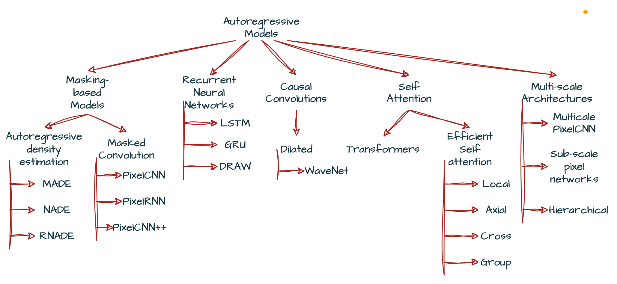
Taxonomy of Autoregressive Models
In the above figure we have tried to do as many plausible classifications of Autoregressive models, there can be more but in the community these are the important ones.
We are no going to learn any of those methods in this blogpost. In future, links to published blogs corresponding to those methods will be added here as list and you can access them directly. This will ease up the navigation process then may it be you want to access root(like in trees) blog post of Generative Modelling: Stormbreaker 🪓 in AI world series or any leaf blog post like LSTM.
Citation
Cited as:
Garg, P. (2023, May 2). Autoregressive Models: Connecting the Dots. Eulogs. Retrieved May 2, 2023, from https://www.eulogs.com/posts/autoregressive-models-connecting-the-dots/
or
|
|
References
[1] Pieter Abbeel. (2020, February 5). L2 Autoregressive Models – CS294-158-SP20 Deep Unsupervised Learning – UC Berkeley, Spring 2020 [Video]. YouTube. https://www.youtube.com/watch?v=iyEOk8KCRUw
[2] Tae, J. (2020a, March 9). Jake Tae. MLE and KL Divergence. https://jaketae.github.io/study/kl-mle/
[3] Tomczak, J. M. (2022). Deep Generative Modeling. Springer Nature
[4] Bond-Taylor, S., Leach, A., Long, Y., & Willcocks, C. G. (2021). Deep Generative Modelling: A Comparative Review of VAEs, GANs, Normalizing Flows, Energy-Based and Autoregressive Models. IEEE Transactions on Pattern Analysis and Machine Intelligence, 44(11), 7327–7347. https://doi.org/10.1109/tpami.2021.3116668