Through this blogpost we are going to gain in-depth understanding of Generative Models, why we need them, along with current taxanomy. But before diving into the Why?, What? of Generative Models, let us consider a simple example of trained Deep Neural Network(DNN) that classifies images of animals. Although the network is trained so well but adding noise to image could output false classification, even though noise added to image doesn’t change the semantics under human perception. This example indicates that neural networks that are used to parameterize the conditional distribution \(p(y|\textbf{x})\) seem to lack semantic understanding of images. A useful model in real world will not only output probability of correctness of classification for example but will be able to tell its level of uncertainity for the answer.
Why Generative Modelling?
Deep Learning models cannot go on making decision about the problems without understanding the reality, and express uncertainity about surrounding world. Assume we have some two-dimensional data and new data-point to be classified. Now, there are two approaches we can use to solve this problem. First, classifier could estimate the result by modelling conditional distribution \(p(y|\textbf{x})\). Second, we can consider joint distribution \(p(\textbf{x}, y)\) that could be further decomposed as \(p(\textbf{x}, y)=p(y|\textbf{x})p(\textbf{x})\).
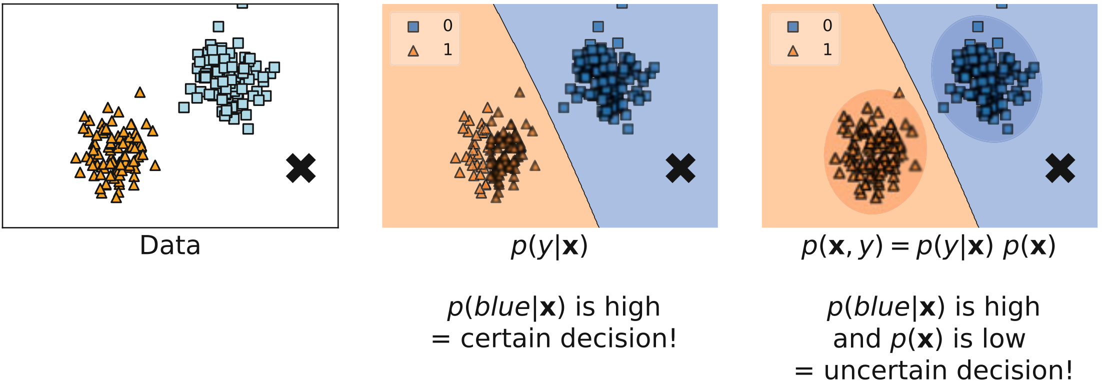
And example of data (left) and two approaches to decision making: (middle) a discriminative approach and (right) a generative approach
In the above figure, both the approaches i.e. discriminative and generative have made a decision boundary. On one hand former is quite certain of “X” being a part of blue region whereas latter uses \(p(\textbf{x})\) to account for additional understanding. Now, “X” lies far from orange zone, but also does not lie in the region of high probability mass in blue zone due to which generative approach said \(p(\textbf{x})\) as low. And, if we want these models to be communicative enough such that as humans we can understand why thy are making decisions that they are making, that would be a crucial skill to exploit.
Significance of p(x)
From the generative perspective, knowing the distribution \(p(\textbf{x})\) is essential because:
- It could be used to assess whether a given object has been observed in past or not.
- It could help to properly weight the decision.
- It could be used to assess uncertainity about the environment.
- It could be used to actively learn by interacting with environment( e.g. by asking for labeling objects with low \(p(\textbf{x})\))
- It could be used to generate (syntheize) new objects.
Though, some if not most of the readers might be ignorant to the use of \(p(\textbf{x})\) only as generator of new data, but above points bring into varied perspectives of it. And at this point, the sail that once started from island of discriminative modelling brought us to the vast land of generative modelling.
Where Can we use (Deep) Generative Modelling?
Deep Generative Modelling need high computational power for training and with the advent of GPU and Deep Learning Frameworks like PyTorch, TensorFlow etc we have seen vast applications thereof.
Some applications vary from typical modalities considered in machine learning:-
- Text Analysis: Question-Answering, Machine Translation, Text-to-Image Generation
- Image-Analysis: Data Augmentation, Super Resolution, Image Inpainting, Image Denoising, Object Transfiguration, Image Colorization, Image Captioning, Video Prediction etc.
- Audio Analysis: WaveNet
- Active Learning: Generate synthetic medical images, generate synthetic text data etc.
- Reinforcement Learning: World Models
- Graph Analysis: Understanding Interaction Dynamics in Social Networks, Anomaly Detection, Protein Structure Modelling, Source Code Generation, Semantic Parsing.
How to Formulate (Deep) Generative Modelling?
After asking some important questions of What and where, its’ time to ask how. In other words we can understand the section heading as how to express \(p(\textbf{x})\). We can divide (Deep) Generative modelling into four categories:- \((1)\) Autoregressive Generative Models(ARM) \((2)\) Flow-based Models \((3)\) Latent variable models \((4)\) Energy-based models
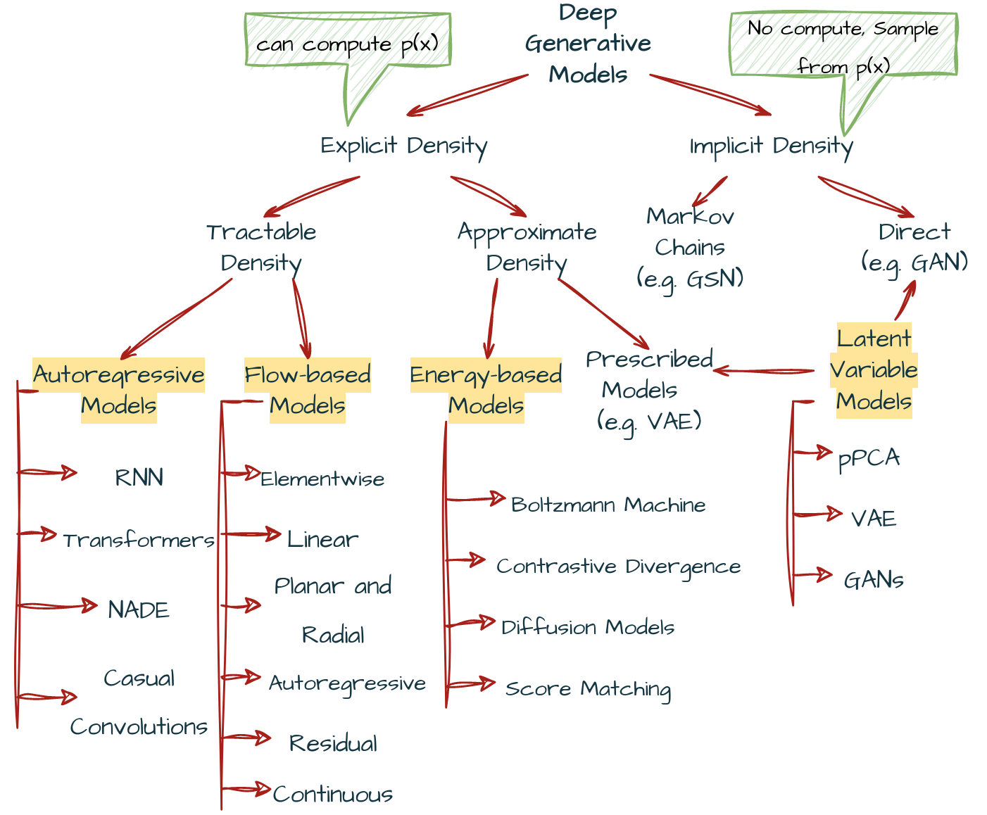
A taxonomy of deep generative models
Deep Generative models can be divided into two types of density estimation methods, namely \((1)\) Explicit Density Models \((2)\) Implicit Density Models. Say you have data distribution \(p_{data}\), \(p_{model}(\textbf{x};\theta)\) likelihood function which learns that data distribution and \(\textbf{x}=[x_{1}, x_{2}, …, x_{n}]^{T}\) are data-points of dataset. Now in explicit density models we compute \(p_{model}(\textbf{x};\theta)\) in short \(p(\textbf{x})\), but in implicit models we dont’ need to compute this likelihood function but directly sample from the distribution e.g. sampling values from noise, and generate for instance image samples using some transformation.
| Explicit Generative Methods | Impliit Generative Methods |
|---|---|
| define an explicit density form(\(p_{model}(\textbf{x};\theta)\)) that allows likelihood inference | target a flexible transformation(Generator) from random noise to generated samples |
| used to estimate the probability density function of the data | can generate new samples from the learned distribution |
| require computing the likelihood of the data, which can be computationally expensive | do not require computing the likelihood |
| typically easier to interpret and analyze | more flexible and can capture complex distributions |
| can suffer from overfitting | can suffer from mode collapse |
| trained using maximum likelihood estimation | typically trained using adversarial training or variational inference |
Explicit Generative Methods
Explicit density methods need to estimate the density of underlying data distribution and marginal likelihood in denominator of bayes rule \(p(z|x)=\frac{p(x,z)}{\int p(x|z)p(z)}\) creates problem since it involves integral. Now if this likelihood can be solved in closed-form expression then those problems lie under tractable density otherwise we need to find approximations to it and so those problems lie under approximate density class. Also, tractable density can be computed in polynomial time but intractable(not approximate) takes more than exponential time to solve. In the given link of Closed Form Expressions a table is given where you can check that we do not have any closed form solution under integral.
Tractable Generative Models
In tractable density models we have two type of techniques namely \((1)\) Autoregressive Models \((2)\) Flow-based Models.
Autoregressive Models
Here, distribution over \(\textbf{x}\) is represented in an autoregressive manner:
$$p(\textbf{x})=p(x_{0})\prod_{i=1}^{D}p(x_{i}\vert\textbf{x}_{<i})$$
where, \(\textbf{x}_{<i}\) denotes all \(\textbf{x}\)’s upto index \(i\).
Modelling all conditional distributions \(p(x_{i}\vert\textbf{x}_{<i})\) would be computationally inefficient. But there are many ways we solve this, although we will not talk about autoregessive models here. Checkout the post Autoregressive Models: Connecting the dots that talk about why we needed these type of models anyway along with its taxonomy.
Flow-based Models
The change of variable formula provides a principled manner of expressing a density of a random variable by transforming it with an invertible transformation \(f\).
$$p(\textbf{x})=p(z=f(x))\vert\text{J}_{f(\textbf{x})}\vert$$
where \(\text{J}_{f(\textbf{x})}\) denotes the Jacobian Matrix.
We can parameterize \(f\) using deep neural networks; however, it cannot be any arbitrary neural networks, because we must be able to calculate the Jacobian matrix. All generative models that take advantage of change of variables formula are referred as flow-based models or flows for short.
Approximate Generative Models
In approximate density models we have two type of techniques namely \((1)\) Prescribed Models \((2)\) Energy-based Models.
Prescribed Models
The idea behind latent variable models is to assume a lower-dimensional latent space and the following generative process: $$\textbf{z} \sim p(\textbf{z})$$ $$\textbf{x} \sim p(\textbf{x}\vert\textbf{z})$$ Latent variables corresponds to hidden factor in data, and the conditional distribution \(p(\textbf{x}\vert\textbf{z})\) could be treated as a generator.
The most widely known known latent variable model is probabilisitc Principal Component Analysis (pPCA) where \(p(\textbf{z})\) and \(p(\textbf{x}\vert\textbf{z})\) are Gaussian distibutions, and dependency between \(\textbf{z}\) and \(\textbf{x}\) is linear.
A non-linear extension of pPCA with arbitratry distributions is the Variational Auto-Encoder (VAE) framework. In VAEs and the pPCA all distributions must be defined upfront and, therefore, they are called prescribed models.
Energy Based Models
Physics provide an interesting perspective on defining a group of generative models through defining an energy function, \(E(\textbf{x})\), and, eventually the Boltzmann distribution: $$p(\textbf{x}) = \frac{e^{-E(\textbf{x})}}{Z}$$ where \(Z=\sum_{\textbf{x}}e^{-E(\textbf{x})}\) is the partition function. \(Z\) normalizes the values of function.
The main idea behind EBMs is to formulate the energy function and calculate(or rather approximate) the partition function.
Implicit Generative Methods
GANs
Above all described methods except EBMs used log-likelihood function for density estimation, but another approach uses adversarial loss where discriminator \(D(\cdot)\) determines a difference between real data and synthetic data provided by the generator in the implicit form, these are Generative Adversaial Networks(GANs) under implicit models.
Overview
Below is provided a table that shows comparision of all the four groups of methods on some arbitrary criteria like:-
- Whether training is typically stable?
- Whether it is possible to calculate likelihood function?
- Whether one can use a model for lossy or lossless compression?
- Whether a model can be used for Representation Learning?
| Generative Models | Training | Likelihood | Sampling | Compression | Representation |
|---|---|---|---|---|---|
| Autoregressive | Stable | Exact | Slow | Lossless | No |
| Flow-based | Stable | Exact | Fast/Slow | Lossless | Yes |
| Implicit | Unstable | No | Fast | No | No |
| Prescribed | Stable | Approximate | Fast | Lossy | Yes |
| Energy-based | Stable | Unnormalized | Slow | Rather not | Yes |
Citation
Garg, P. (2023a, April 30). Generative Modelling: Stormbreaker 🪓 in AI world. Eulogs. Retrieved May 2, 2023, from https://www.eulogs.com/posts/generative-modelling/
or
|
|
References
[1] Tomczak, J. M. (2022). Deep Generative Modeling. Springer Nature
[2] Wu, Q., Gao, R., & Zha, H. (2021). Bridging Explicit and Implicit Deep Generative Models via Neural Stein Estimators. In Neural Information Processing Systems (Vol. 34). https://papers.nips.cc/paper/2021/hash/5db60c98209913790e4fcce4597ee37c-Abstract.html
[3] Bond-Taylor, S., Leach, A., Long, Y., & Willcocks, C. G. (2021). Deep Generative Modelling: A Comparative Review of VAEs, GANs, Normalizing Flows, Energy-Based and Autoregressive Models. IEEE Transactions on Pattern Analysis and Machine Intelligence, 44(11), 7327–7347. https://doi.org/10.1109/tpami.2021.3116668