Life is not complex. We are complex. Life is simple, and the simple thing is the right thing.
Over the span of last decade, Deep Learning has made our life simpler by bringing its power into the applications of healthcare, self-driving cars, fraud-prevention and many more. Since the launch of ChatGPT many companies have made applications which help users in brainstorming and simplifying comlpex ideas, assist in writing content, even assist in writing codes etc. Their predictive analysis power depends on the assumption that these models are learning what we intend them to learn, e.g. to classify a cow, model must be looking at cow and not at grass. But has it been the case the whole time?
Introduction
Lets’ start with an example of Bob and Alice who are studying for high school exams. Bob used a strategy of mugging up while Alice likes to understand things in detail and then ponder over it. Bobs’ strategy got him good grades in test unlike Alice, but can Bob extrapolate/generalize this strategy in order to apply the learned concepts to real world applications like Alice. Alice can use her strategy almost anywhere in life and would benefit from it but Bob will fail in the wild. Bob has taken shortcut to complete the task instead of actually learning principles. But are these shortcuts bad? When human driver takes shortcut route to reach destination its good for you since it saved time. So it depends on the type of task we are doing and also the context of it to determine taking shortcut is okay or not.
We are using Deep Learning techniques especially for the field of computer vision in self drving cars, security cameras, activity recognition etc on daily basis. But even after 5 decades we haven’t really understood the underlying principles behind the success of these models. Only on the basis of test performances we are deploying them in the wild. Since they are being used as applications in court, defence, person identification etc which makes the need to understand them necessity than leaving it as another field of scientific endeavour[1].

|

|
|
|
|---|---|---|---|
| Task | Image Captioning | Recognize Pneumonia | Answer Question |
| Problem | Describe scene as grazing sheep | Fails on scans from new hospital | Changes answer if irrelevant information is added |
| Shortcut | Uses background(hillside) to recognize primary object | Looks at hospital token, not lungs | Only looks at last sentence and ignores context |
In the above table Deep Neural Nets are often solving problems taking shortcuts instead of learning the core features. This is prevalent but not only limited to the field of deep learning, infact humans and animals also tend to take shortcuts as we saw an example in the starting of Introduction. These shortcuts tend to work well for confined space but do not generalize well in the real world. For e.g. Amazons’ DNN model made hiring decision on basis of resume, but were biased for men.
This has given rise to the new field of study in Deep Learning called Shortcut Learning. Shortcuts can be understood as spurious features that perform well on standard benchmarks but fail to generalize to real-world settings[2]. Spurious features are features that were used during training(e.g. grass) of predictive model e.g classification model but are not useful in general real-world settings(e.g. grass does not imply prediction of cow).
Related Works
The field of shortcut learning is not novel problem, it been there for long time in the field of machine learning with different names
- Learning under Covariate Shift
- Anti-Casual Learning
- Dataset Bias
- Clever Hans Effect
Shortcut learning works like an umbrella term to consolidate all the above terms and likewise under the hood to work on the problem as a whole.
Lets’ start understanding shortcut learning from the biological perspective first.
Shortcut Learning in Biological Neural Networks
Unintended Cue Learning
“In experimental psychology, unexpected failures are often the consequence of unintended cue learning. For example, rats trained to perform a colour discrimination experiment may appear to have learned the task but fail unexpectedly once the odour of the colour paint is controlled for, revealing that they exploited an unintended cue—smell—to solve what was intended to be a vision experiment…1”
Researchers intended the problem to be of vision but rats found the solution by learning the smell of the colors which was unintended by researchers. Though solution worked for given experiment but it will be hard to extrapolate the learnings to other experiments.
Surface Learning
Students’ learning process has been broadly classified into two groups 1. Deep Learning and 2. Surface Learning. Taking the reference of Bob and Alice example, Alice would be deep learner and Bob would be the Surface Learner. Bob was focused on grasping the main points and memorizing them, on the other hand Alice showed interest in the meaning of the topics to deepen the understanding by cross linking the learnings with other knowledge. This aid deep learners to transfer their learning strategy to other topics of study or not just subject matter but also to real life dealings. Analogy to machine learning can be, Transfer Learning. Bobs’ transfer learning is highly intended to fail on other topics unlike Alices'.
Example showing the decision rules of Shortcut Learning
Any machine learning or deep learning model apply decision rules in order to categorize or predict or do any such tasks on a dataset. This defines a relationship between input and output of the model. In this section we will take the example from [1]
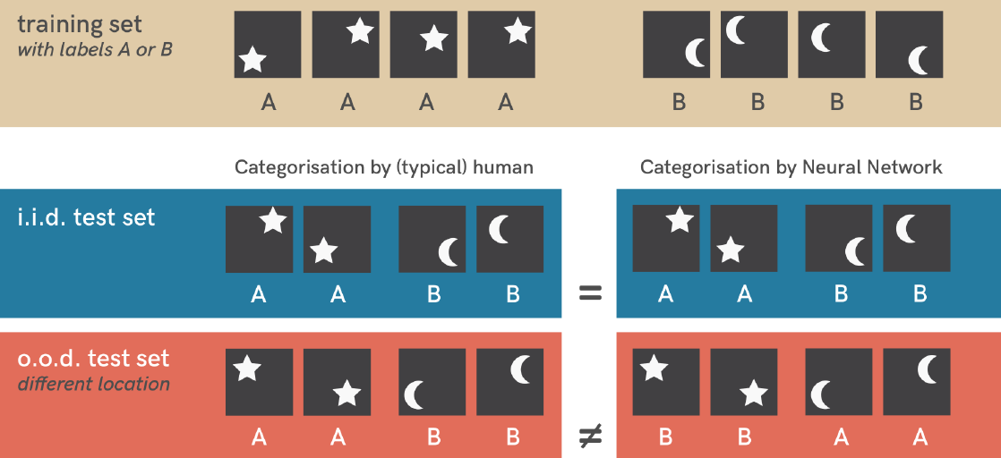
In the above figure, we are given a dataset containing two categories(star ⭐ , crescent 🌙) with labels A, B respectively. In the machine learning we usually divide the dataset into training set and test set in some proportion say 80:20 or if the number of datapoints are large then 90:10. Also our datasets usually follow some distribution class wise e.g images of cow would be mainly found in grassfields. Now after dividing the dataset into train and test sets we get i.i.d which is identically independent distribution, think of it as a subset sampled from the dataset. Such that this subset follows the same distribution as dataset. But when only some part of dataset is taken in consideration to make a subset e.g. cow is taken as object of interest, but we change the conditions in which those objects are existing e.g. cow on road instead on grassland. Then this is o.o.d which is out of distribution.
After the model has been trained on the train set, its been tested on i.i.d subset where location of classes seemed to have not changed. Because of which Neural Network model were able to classify them correcty. But, why location? why not shape?. For that we used o.o.d subset in which we changed the location of classes and neural network model failed to classify it correctly. If it would be learning the classification on the basis of shapes which is intended feature then it would have answerd correctly. Wrong classification shows that it learned the location of classes in order to classify which is spurious feature.
Where do these shortcuts come from?
Principle of Least Effort
Phenomenon of “Principle of Least Effort” came from the field of lingustics where speakers tend to minimize the amount of effort involved in communication. E.g. speaking “plane” instead of “airplane”, merging “p” and “b” in “cupboard”. Related analysis can be found in Morgans’ Canon, Monitoring Early Training Dynamics.
Skewed Training Dataset
Today we mostly use crowd-sourcing platforms like Amazon Mechanical Turk for labeling in vision data, annotating in language data etc for its low cost and scalability. But this comes with its’ own price of biases and artifacts due to collection bias. Since labelling and annotating datapoints are not done by single entity, this entails individual biases from annotators. For e.g. in NLI task, annotators have usually written contradiction by using not and this created a spurious feature for language model to base its predictions on. Now these annotations are not wrong, but we need robust models to handle this type of bias.
Neural Network Models
In LLMs its been seen that two factors are important in order to determine the models’ robustness. (1) Model Size (2) Pre-training objective
Model Size
Model size is measured by number of parameters while keeping the kind of architecture and pre-training objective same. Now generalization ability is measured by the performance of model on o.o.d dataset. Its been shown that generalization ability of larger models are better than those of smaller ones, also smaller models are prone to capture spurious features and more dependent on data artifacts for prediction [5]. For e.g. BERT-large will generalize better than BERT-base. Following this we can also talk about model compression, a theoritical perspective has shed some light by showing that there is a tradeoff between size of model and robustness[7]. Empirically its also been found that compressing the LLM reduces the robustness and especially the models that have been compressed using knowledge distillation are more vulnerable to adversarial attacks.
Pre-training Objectives
Lets’ take 3 kinds of LLMs: BERT, ELECTRA, and RoBERTa,. Now for Adversarial NLI dataset, ELECTRA and RoBERTa have better performance than BERT. Similarly, its’ been shown that RoBERTa-base outperformed BERT-base on HANS test by 20%. Also empirical evidence show that above three models have different levels of robustness most probably because of inductive bias as pre-training objective.
Dataset Bias
Lets’ take an example of penguin. What makes penguin a penguin? Penguin itself or the context, ofcourse penguin itself but context helps for increasing the probability of correctness. But if only context becomes more important than object itself, that’s a problem. If we have penguin in snow data mostly, then strategy of classifying snow as penguin becomes successful even when penguin would not be there. Indeed many models base their predictions on context than object itself and this creates shortcut opportunity for models.
To deal with these dataset biases researchers proposed to scale up the dataset size in order to have sufficient samples with more diversification. Consequently even large real world datasets like Imagenet are highly influenced by it [4]
Discriminative Learning
Generally it is sufficient for discriminative model to rely on textures and local structures for object classification. But in generative modelling model needs to understand the global shape of object also and not just textures for generating human understandable images. Model is better off learning the textures and ignoring the shape bias for learning object classification task and that becomes a problem e.g. dog image may have the texture of elephant but humans would be classfying the image on the basis of shape rather than texture.
Standard DNNs are intended to learn some workable relationship between input and output and not explicitly take the human interpretability factor of the following relationship into consideration. This ease of finding relationship severly bias the model to learn overly simplistic solutions which perform well on standard benchmarks but fail in real world[1].
Shortcut Learning across Deep Learning
Computer Vision
Slight changes in the translation, rotation, adding noise, changing background of the object in the image has shown to derail the predictions of DNNs. Models learn shortcuts that are inherent to the distribution of the dataset because of which these models do not perform well when used as transfer learning. Since they have learned the representations which will only work in limited capability under distribution shift. Tiny invisible changes to human eye in the images can alter the predictions of neural network by great margin. This is an example of Adversarial Learning which is one of the most severe failure cases of neural networks[1]
Natural Language Processing
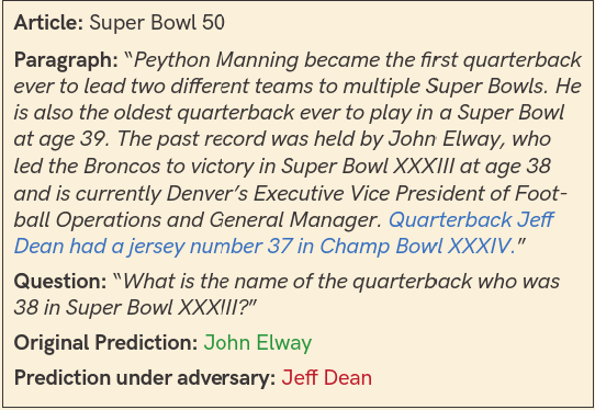
Studies have found that Large Language Models (LLMs) are vulnerable to adversarial attacks and have low generalization power[5]. Empirical Analysis shows that BERT-like models base their performance of Natural Language Inference (NLI) task on some spurious features like unigrams not, do, is and bigrams will not. Some models were relying on lexical matching of words between question and original passage in reading comprehension task, which tend to ignore the understanding of comprehension. Natural Language Understanding (NLU) dataset contains artifacts and biases, due to which LLMs using training strategy of Empirical Risk Minimization (ERM) have learned to rely on spurious correlations of them and class labels.
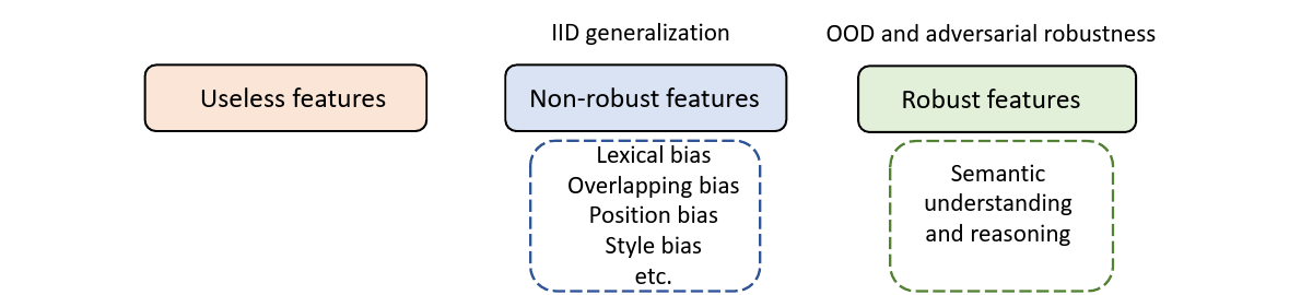
Now features learned by the model can be broadly classified into three categories: (1) Useless Features (2) Non-robust Features (3) Robust Features. Shortcut Learning can also be understood as a phenomenon that rely highly on non-robust features. These type of features are aligned with biases in training data. Below figure may help in providing better understanding at it.
-
Lexical Bias: Some lexical features like stop words, numbers, negation words have high correlation of co-occurence with certain class labels. E.g. LLMs tend to give contradiction predictions whenever there exist negation words e.g. never, no in input
-
Overlap Bias: Reading comprehension models use the overlap/lexical matching between passage and question pair for prediction rather than understanding underlying task. Similarly, Question Answering (QA) models perform by relying on heuristics of question and context(knowledge base) lexical matching.
-
Position Bias: Lets understand this using an example, take the QA task where answers to most of the questions lie in the kth line in each passage. This will make QA model to use position cues as spurious feature for prediction.
-
Style Bias: LLMs have leared to rely on spurious text styles as shortcuts. These features can be further utilized as backdoor attacks for adversarial pertubations to decrease models’ robustness.
Fairness and Algorithmic Decision-Making
Amazon trained a deep neural network to filter out strong candidates for a job on the basis of resumes, but later it was found out to be gender biased towards men. Gender was such a strong predictor that even after removal of that attribute from dataset, model always found a way around, e.g. inferring gender from all-woman college names. When human biases are not only replicated, but worsened by a machine, this is referred to as bias amplification[1]. Amplification of disparity among groups over time is referred to as disparity amplification. Example regarding latter can be a shortcut feature that focus on majority group in dataset than underrepresnted.
Identification of Shortcut Learning
Comprehensive Performance Testing
-
We need to test models on o.o.d datasets to understand if the model has learned the features that we are interested in. HANS (Heuristic Analysis) evaluation set is proposed to evaluate whether NLI models have syntatic heuristics: the lexical overlap heuristic, the subsequence heuristic, the constituent heuristic. Following the philosophy of HANS, a new task has been created: FEVER for facts verification[5]. These o.o.d tests have shown performance degradation for State-of-the-art Large Language Models.
-
Adversarial Attacks makes an interesting diagnostic tool. If a successful and innocuous adversarial attack can change the predictions of model without changing semantic content, then this is indicative of presence of a shortcut.
-
Ablation studies are useful in order to understand what essential factors are contributing to models performance. Recent ablation studies show that word order does not matter for pre-trained language models. This points out to the fact that LLMs success relies on the ability to understand the correlation between the word co-occurences no matter where words lie in a sentence.
Explainability Analysis
Deep Neural Networks are black boxes which employs a limitation to understand the decision process. Explainability methods are helpful in those scenarios in order to provide some useful insights into the working of DNNs.
Feature Attribution
-
Assume you have an input \( x \) for NLP task, then \( x_{i}\) implies each token. Feature Attribution algorithm \(\Phi\) will calculate \(\Phi_{i}\) which denotes the contribution score of \(x_{i}\) for model prediction.
-
The tokens in the training set can be modeled using long-tail distribution. This can create a shortcut for LLM to concentrate biasedly towards the head of the distribution even though tail of the distribution has abundant information.
Instance Attribution
You are what you eat
The following quote also applies to Deep Neural Networks except they consume data and then base their prediction. Every preceding datapoint affect the prediction of sucessive sample in dataset. Instance Attribution methods are useful in predicting the data samples that contributed more to the models’ prediction performance for particular instance/datapoint. Empirical analysis indicates that the most influential training data share similar artifacts e.g. high overlapping bias between premise and hypothesis for NLI task.
Morgans’ Canon for Machine Learning
Psychologist Lloyd Morgon developed a guideline for interpreting non-human behaviour in response to the fallacy of Anthromorphism.
Morgons’ Canon says that “In no case is an animal activity to be interpreted in terms of higher psychological processes if it can be fairly interpreted in terms of processes which stand lower on the scale of psychological evolution and development”
Simple correlation would be considered low on psychological scale than scene understanding. Morgons’ canon in terms of machine learning can then be “Never attribute to high-level abilities that which can be adequately explained by shortcut learning”
Morgons’ canon can also be understood as Occams’ Razor that says “It is futile to do with more what can be done with fewer”. A small patch added to image at certain location for all the images of the class is enough for the model to base its predictions and, complex objects and textures of say some animal would not even be needed for it to classify.
Monitoring Early Training dynamics
Up until now, community has viewed shortcut learning as a distribution shift problem, but [2] formalized the guideline of Morgons’ Canon to show difficulty of spurious feature is equally important in order to understand or identify shortcuts. They argued that it can be captured by monitoring early training dynamics, think of monitoring training dynamics as observing the changes of neural network predictions, maybe weights or any likewise insight during the course of training.
Premises that support the hypothesis: “Difficulty of spurious features is important for shortcut learning”
- Shortcuts are only those spurious features that are easier to learn than the intended features.
- Initial layers of DNN learn easy features or low level features, whereas later layers tend to learn harder ones or high level features.
- Easy features are learned much earlier than the harder ones during training [6]
lets solve the premises using propositional logic, for ease we will use \(premise_{n} \rightarrow p_{n}\)
| \(p_{1}: S\) | \(p_{2}: I \land L\) | \(p_{3}: E \land H\) |
| \(S:\) “Shortcuts are easy features” | \(I: \) “Initial layers learn easy features” | \(E: \) “Easy features are learned earlier during training” |
| \(L: \) “Later layers learn hard features” | \(H: \) “Hard features are learned later during training” |
conjuction of \(p_{2}, p_{3}\) \(= p_{2} \land p_{3} = I \land L \land E \land H = (I \land E) \land (L \land H)\)
we are only concerned with easy features (\(I\)) rather than hard features, since spurious features are easier to learn. So \(L \land H\) can be removed from above equation.
then, \(p_{1} \land p_{2} \land p_{3} = S \land I \land E\)
This leads to conjecture, “Shortcuts are easy features that are learned by initial layers early during training”
Now we need to define the notion of task difficulty(\(\Psi\)) which actually depends on model and data distribution (\(X, y\)) where \(X\) is input and \(y\) is label. Then \(\Psi_{M}^{P}(X \rightarrow y)\) indicates difficulty of predicting label \(y\) given input \(X\) for model \(M\) and some distribution \(P\), where \(X, y \sim P\). Spurious feature \(s\) is potential shortcut for model \(M\) iff \(\Psi_{M}^{P_{tr}}(X \rightarrow y) > \Psi_{M}^{P_{tr}}(X \rightarrow s)\). Which means, difficulty of predicting spurious feature \(s\) is easier than predicting label \(y\) for model \(M\) for a training distribution \(P_{tr}\).
But how would we measure the task difficulty? using two metrics Prediction Depth and \(\nu\)-Usable Information. Prediction Depth of an input is defined as minimum number of layers required by the model to classify the input. \(\mathit{\boldsymbol{\nu}}\)-Usable Information is defined as amount of usable information in some input \(X\) that can be used by model to predict \(y\), higher the usable information easier the dataset or datapoint/sample is.
We are close to the end of this section, hold tight. Now consider two datasets \(D_{s} \sim P_{tr}(X, y)\) with spurious features and \(D_{i} \sim P_{te}(X, y)\) without spurious features. Taking some assumptions in Prediction Depth (PD) if mean PD of \(D_{s}\) is less than mean PD of \(D_{i}\) then \(\nu\)-Usable Information for \(D_{s}\) is higher than for \(D_{i}\). In such scenerio model will tend to learn spurious features than intended ones. And this can help to identify spurious features.
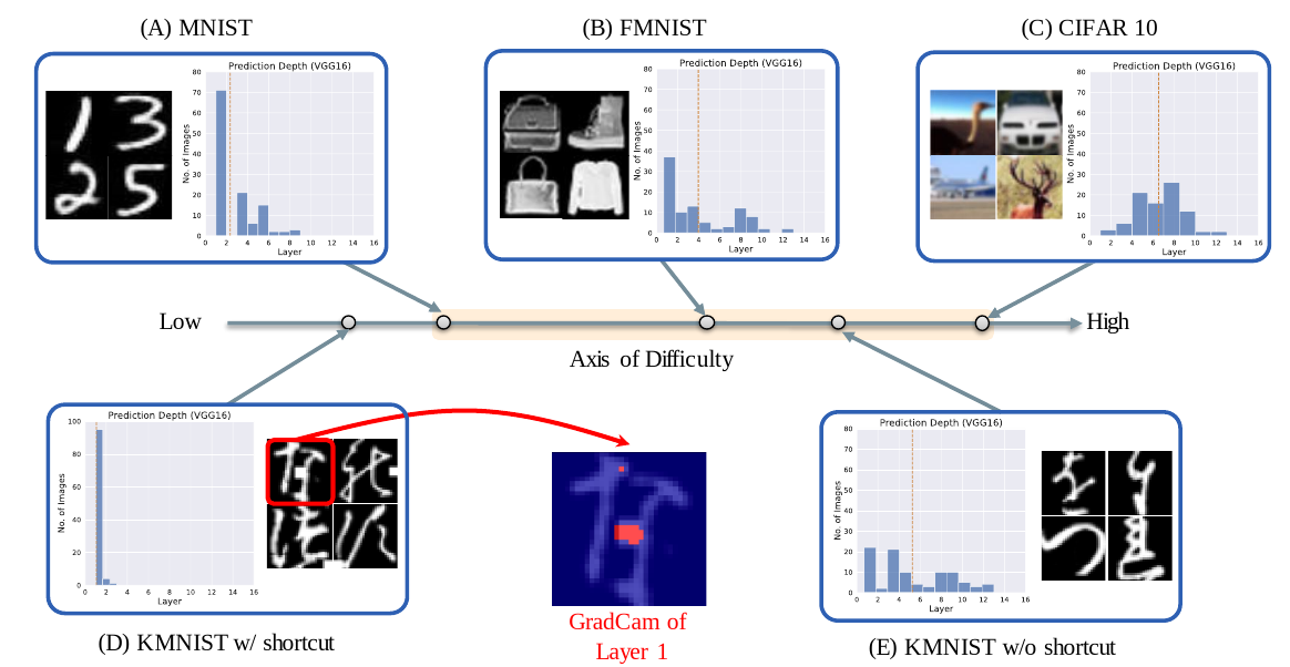
Datasets lying on the mean PD axis in order of difficulty. KMNIST with shortcut has least difficulty due to the introduction of shortcut whereas KMNIST with no shorcut is even difficult than FMNIST
Mitigation of Shortcut Learning
Dataset Refinement
The aim of dataset refinement is alleviating biases from training datasets. There are some ways using which we can alleviate biases.
-
By providing additional instructions to crowd workers to drop down the use of words that are highly indicative of annotation artifacts.
-
Using Adversarial Filtering to filter out the bias in dataset. Models trained on these debiased datasets have to learn more generalizable features and rely on common sense reasoning.
-
Using data augmentation methods like counterfactuals, MixUp, CutPaste, rotation and many more can be helpful in debiasing.
Adversarial Training
This is implemented in two ways:
-
Task classifier and adversarial classifier jointly share the same encoder and the goal of the adversarial classifier is to provide correct predictions for the artifacts in training data.
-
Model is trained to minimize the loss function over generated adverarial examples but such techniques haven’t shown much generalization abilities.
Many techniques like \(l_{1}\), \(l_{2}\) regularization, CutOut, MixUp and early stopping have been investigated, where early stopping is found to be most effective.
Product-of-Expert(POE)
This provides us with an opportunity to model high dimensional data by combining some low dimensional models, where every low dimensional model will focus on some particular constraint of the problem by giving high probability. Since our goal is to debias the model, we can follow two stage system to achieve this.
- In first stage, bias-only model is trained to capture bias of the dataset.
- In second stage, debiased model will be trained using cross-entropy loss and only the weights of debiased model will be updated.
In this way debiased model will use the information from biased model to improve its predictions.
Training Samples Reweighting
This is also known as worst group loss minimization. The main idea of the following technique is to assign higher weight to hard training examples in a batch. This is because model tend to learn easy features more than hard ones and so improving the performance of worst group (hard samples) is beneficial for model robustness. [8] used a combination of Low Capacity Network (LCN), and High Capacity Network (HCN) for reweighting the data samples.
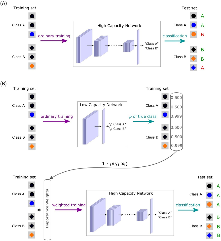
We know easy features are learned in early layers of neural network according to Prediction Depth Analysis we did above. LCN can then very well capture those features by been trained to fit to the dataset such that it will give high probabilities for spurious or here easy featues. These probabilities can then be used to reweight the samples that are hard such that model will focus more on hard samples to find relevant and hopefully intended features to learn underlying distribution of the dataset. Imbalance Dataset problem can also be part of this section which researchers of Meta tried to solve by introducing focal loss.
Contrastive Self-Supervised Learning
Contrastive Learning comes as a subset to Representation Learning which aims to learn better representations by creating auxillary tasks that eventually help the model to perform better on main task or say downstream tasks like classification. Constrastive Learning methods usually suffers with feature suppression, say you have two images of one is dog running on a sunny day and another is cat standing still under shade. Model will discriminate both on the basis of sunny and shady supressing other intended features. So auxillary tasks need to created very carefully keeping problems of feature suppression in account.
Introducing Challenging Evaluation Datasets
Adversarial GLUE is proposed for adversarial robustness evaluation which contains 14 adversarial attack methods. Similary Checklist, Robustness Gym can be used to evaluate the robustness of LLMs. Introduction to datasets that contain wide range of tasks, biases and so on can give better insights about Deep Neural Nets performance. [4] introduced Spurious ImageNet which consists of 40 spurious features and each consists 75 images, images didn’t had any class objects like car, animal, object but just spurious features. This allowed to check the influence of unintended features over the performance for any vision model.
Conclusion
Every shortcut has a price usually greater than the reward
Applications powered using Deep Learning are taking world by storm but under the light of aid that these models are providing us, we shall not unlook the fundamental working principle of these models. Shortcut Learning rather being taken as another problem in the field of Neural Nets, it should be considered default for performance comparision and to better understand what our neural net is actually learning. Overcoming shortcut learning will help in solving fairness, robustness, deployability and trust worthiness of these models. This will eventually make machine decisions more transparent.
Citation
Cited as:
P. Garg, “Shortcut Learning: Belief trap of Deep Neural Networks,” Eulogs, Mar. 31, 2023. https://www.eulogs.com/posts/shortcut-learning/ (accessed Apr. 13, 2023).
or
|
|
References
- Geirhos, Robert, et al. "Shortcut learning in deep neural networks." Nature Machine Intelligence 2.11 (2020): 665-673
- Murali, Nihal, et al. Shortcut Learning Through the Lens of Early Training Dynamics. 1, arXiv, 2023, doi:10.48550/ARXIV.2302.09344
- Geirhos, Robert, et al. “Unintended Cue Learning: Lessons for Deep Learning from Experimental Psychology.” Journal of Vision, vol. 20, no. 11, Association for Research in Vision and Ophthalmology (ARVO), 20 Oct. 2020, p. 652. Crossref, doi:10.1167/jov.20.11.652.
- Neuhaus, Yannic, et al. Spurious Features Everywhere -- Large-Scale Detection of Harmful Spurious Features in ImageNet. 1, arXiv, 2022, doi:10.48550/ARXIV.2212.04871.
- Du, Mengnan, et al. Shortcut Learning of Large Language Models in Natural Language Understanding: A Survey. 1, arXiv, 2022, doi:10.48550/ARXIV.2208.11857.
- Karttikeya Mangalam and Vinay Uday Prabhu. Do deep neural networks learn shallow learnable examples first? 2019.
- Bubeck, Sébastien, and Mark Sellke. A Universal Law of Robustness via Isoperimetry. 4, arXiv, 2021, doi:10.48550/ARXIV.2105.12806.
- Dagaev, Nikolay, et al. “A Too-Good-to-Be-True Prior to Reduce Shortcut Reliance.” Pattern Recognition Letters, vol. 166, Elsevier BV, Feb. 2023, pp. 164–171. Crossref, doi:10.1016/j.patrec.2022.12.010.