Science does not aim at establishing immutable truths and eternal dogmas; its aim is to approach the truth by successive approximations, without claiming that at any stage final and complete accuracy has been achieved.
Motivation
Lets’ recall the Bayes theorem that most of us might already be familiar with, it goes like $P(A \vert B) = \displaystyle \frac{P(B \vert A)P(A)}{P(B)}$. Here, $P(B \vert A)$ is conditional probability which can be interpreted as likelihood function or probability density function if working with continuous system else probability mass function. $P(A)$ is prior probability which is assumed probability distribution of the system before any evidence is taken in account. $P(B)$ is marginal probability which is used as a normalizing quantity. All the recently mentioned quantities are used to inference(reaching conclusion on the basis of evidence and reasoning) about posterior $P(A \vert B)$.
In bayesian models, we use latent(hidden) variables which govern the distribution of data. We can write these latent variables as $z$ and data (say for images) as $x$. Now bayes theorem will become $P(z \vert x) = \displaystyle \frac{P(x \vert z)P(z)}{P(x)}$, in words it would mean that we have currently assumed some prior distribution over latent variables(e.g. standard normal) multiplying it with likelihood function of getting desired image $x$ for fixed latent variable $z$ and normalizing it with marginal probability of finding desired image out of all plausibilities as $P(x)$. We know prior distribution because we are assuming it, so we may sample from it too and this would make likelihood function to be tractable too since we know $x$, $z$. But quantity that brings hinderance to solving posterior is marginal probability, since we have no realization that how many possible values of $x$ may exist such that we cannot find the probability of getting desired image $x$ out of all plausibilities.
So, we need to talk about the problem of marginal probability distribution here, lets’ expand the formulation in terms of joint probability.
$$ \begin{align} P(x) = \int_{z} P(x, z) \ dz \label{eq:1}\tag{1} \end{align} $$
Equation (\ref{eq:1}) says that marginal probability is equal to integration of joint probability over all the values of $z$, though we have prior on $z$ but its’ an assumption and so it may happen that we dont’ get all the values for $z$, and in that case our integral will not be in closed form which in turn will not give exact value of integral and we would need to approximate. One of the core problems of modern statistics is to approximate difficult-to-compute probability densities.
Introduction
There are various methods for solving approximation problems, one of them is variational inference (VI), which is widely used to approximate posterior densities for Bayesian models. But theres’ an alternative to that, Markov Chain Monte Carlo (MCMC) sampling. We will talk briefly about MCMC and see why these methods are not optimal to work with for most machine learning tasks.
Markov Chain Monte Carlo
MCMC approaches have grown in popularity during the past few decades. These are computer-driven sampling approaches that allow one to describe the nature of a distribution without understanding its mathematical properties by randomly sampling out the data.
The word MCMC is a combination of two properties: Monte-Carlo and Markov chain. Monte Carlo is the practise of estimating the parameters of a distribution by studying random samples from the distribution. For example, instead of simply computing the mean of a normal distribution from its equations, a Monte Carlo technique would be to pick a large number of random samples from a normal distribution and compute the sample mean of them. This advantage is most noticeable when drawing random samples is simple, and distributions’ equations are hard to work with.
The notion behind MCMC’s Markov chain property is that random samples are generated via a particular sequential process. Each random sample serves as a stepping stone for the generation of the next random sample (thus the chain). The chain has a unique characteristic in that, while each new sample depends on the one before it, new samples do not depend on any samples before the prior one (this is known as the “Markov” property) [2].
In MCMC, we first construct an ergodic Markov chain on $z$ whose stationary distribution is the posterior $P(z | x)$. Then, we sample from the chain to collect samples from the stationary distribution. Finally, we approximate the posterior with an empirical estimate constructed from (a subset of) the collected samples [1].
Benefits
- Indispensible tool to modern bayesian statstics
- Landmark developments like:-
- Metopolis-Hastings Algorithm
- Gibbs Sampler
- Hamilton Monte Carlo
- Provide guarantees of producing asymptotically exact samples from target density.
MCMC have been widely studied, extended and applied to more than field of statistics but even to psychology.
Limitations
But, alas, every rose has its’ thorn.
- Sampling speed slows down as size of datasets or complexity of models increases.
- Computationally more intensive than Variational Inference
- For mixture models, MCMC sampling approach of Gibbs Sampling is not an option even for small datasets
This is why, MCMC is suited to smaller datasets and scenerios where we pay heavy computational cost for more precise samples.
Variational Inference
The key idea behind the variational inference is to approximate a conditional density or posterior of latent variables given observed variables $P(\textbf{z} \vert \boldsymbol{x})$. Its’ important to note that we dont’ approximate with single datapoint or sample but with arbitrarily many. So $\boldsymbol{x} = x_{1:n}$ be set of $n$ observed variables and $\textbf{z} = z_{1:m}$ be a set of $m$ latent variables. In the motivation section we have already set the stage for describing the problem with Bayesian theorem.
Bayesian Mixture of Gaussians
Consider a mixture of univariate Gaussians having unit-variance $(\sigma^{2} = 1)$ and $K$ mixture components.
Means $\boldsymbol{\mu} = \lbrace \mu_{1},…,\mu_{K} \rbrace$ for \(K\) Gaussian distributions. These mean values are sampled independently from common prior density $P(\mu_{k})$, which is assumed to be Gaussian $\mathcal{N}(0, \sigma^{2})$ where $\sigma^{2}$ is hyperparameter.
To generate an observation $x_{i}$ from the model, we first need to choose cluster assignment $c_{i}$, which is an indicator function that indicates from which cluster $x_{i}$ comes. It is sampled from categorical distribution over $ \lbrace 1,…,K \rbrace $ since we have $K$ clusters. So its’ $\displaystyle \frac{1}{K}$ probability for $c_{i}$ to choose any cluster. Every $x_{i}$ will have corresponding $c_{i}$, and $c_{i}$ will itself be $K$ dimensional. For e.g. $c_{i} = [ 0,0,0,1,0,0 ]$, this indicates that $x_{i}$ belongs to $4^{th}$ cluster out of $K=6$ clusters.
Every cluster will be of following probability density; $\mathcal{N}(c_{i}^{T}\boldsymbol{\mu}, 1)$.
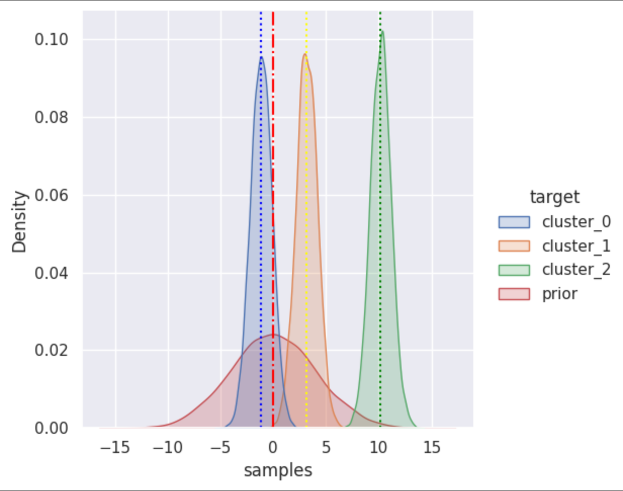
In this visualization red color of gaussian distribution is prior density with σ=4 and µ=0. Three random values are sampled from prior as means of other three distribution in color green, yellow and blue with σ=1. Vertical line shows the mean of each distribution.
Full hierarchical model is, $$ \begin{align} \mu_{k} &\sim \mathcal{N}(0, \sigma^{2}) & k &= 1,…,K \label{eq:2}\tag{2} \cr c_{i} &\sim Categorical(\frac{1}{K},…,\frac{1}{K}) & i &= 1,…,n \tag{3} \cr x_{i} \vert c_{i}, \boldsymbol{\mu} &\sim \mathcal{N}(c_{i}^{T}\boldsymbol{\mu}, 1) & i &= 1,…,n \label{eq:4}\tag{4} \end{align} $$
$c_i$ is independent of $c_j$ where $i \ne j$ and this makes $x_i$ only dependent on $c_i$, so joint density of latent and observed variables for $n$ data samples will be,
$$ \begin{align} P(\boldsymbol{z, x}) &= P(\boldsymbol{\mu, c, x}) & \cr &= P(\boldsymbol{x}\vert\boldsymbol{c,\mu})P(\boldsymbol{c}\vert\boldsymbol{\mu})P(\boldsymbol{\mu}) \cr &= P(\boldsymbol{x}\vert\boldsymbol{c,\mu})P(\boldsymbol{c})P(\boldsymbol{\mu}) \tag{5} \cr P(\boldsymbol{\mu}, c_{1},…,c_{n},x_{1},…,x_{n}) &= P(\boldsymbol{\mu})P(x_{1},…,x_{n}\vert c_{1}, …, c_{n}, \boldsymbol{\mu}) \cr & \qquad P(c_{1},…,c_{n}) \cr &= P(\boldsymbol{\mu})\prod_{i=1}^{n}P(c_{i})P(x_{i}\vert c_{i}, \boldsymbol{\mu}) \label{eq:6}\tag{6} \end{align} $$
Note that $\boldsymbol{\mu}$ though independent, has not been decomposed to independent $\mu_k$ like $\boldsymbol{c}$, since $x_i$ can be sampled from any of $K$ clusters. This is why we cannot decompose the $\boldsymbol{\mu}$. We took latent variables $\boldsymbol{z}={\boldsymbol{\mu},\boldsymbol{c}}$. Now evidence is,
$$ \begin{align} P(\boldsymbol{x}) &= \int_{\boldsymbol{\mu}}\int_{\boldsymbol{c}}P(\boldsymbol{\mu})\prod_{i=1}^{n}P(c_{i})P(x_{i} \vert c_{i}, \boldsymbol{\mu}) \ d\boldsymbol{c} \ d\boldsymbol{\mu} \cr &= \int_{\boldsymbol{\mu}} \sum_{j=1}^{n}P(\boldsymbol{\mu})\prod_{i=1}^{n} P(c_{j})P(x_{i}\vert c_{j}, \boldsymbol{\mu}) \ d\boldsymbol{\mu} \cr &= \int_{\boldsymbol{\mu}} P(\boldsymbol{\mu}) \prod_{i=1}^{n} \sum_{j=1}^{n} P(c_{j})P(x_{i} \vert c_{j}, \boldsymbol{\mu}) \ d\boldsymbol{\mu} \tag{7} \end{align} $$
Time complexity of numerically evaluating the $K$-dimensional integral(since $\boldsymbol{\mu}$ is $K$-dimensional) is $O(K^{n})$. Its’ interesting to note that $\sum$ term will be vectorized and will take one unit computing time, and only $\prod$ term will be left with $n$ as max samples.
So computing the evidence remains exponential in $K$, hence intractable.
Evidence Lower Bound
Recall, that we are facing hardships in evaluating the posterior $P(\boldsymbol{z} \vert \boldsymbol{x})$. Now, the main idea behind variational inference is to approximate this posterior by optimizing the parameters of some family of density function e.g. Gaussian such that it will minimize the KL-Divergence between these two distributions.
$$ \begin{align} q^{*}(\boldsymbol{z}) = \arg \min_{q(\boldsymbol{z}) \in \mathcal{D}} KL(q(\boldsymbol{z}) \Vert P(\boldsymbol{z} \vert \boldsymbol{x})) \tag{8} \end{align} $$
where, $\mathcal{D}$ is a family of densities over latent variables, e.g. Gaussian, Bernoulli, Gamma probability density functions. By $q(\boldsymbol{z}) \in \mathcal{D}$ we are going to choose one family, but every family will have infinite members e.g. Gaussian has hyper-parameters $\mu, \sigma^{2}$ mean, variance respectively and each pair of values of both hyperparameters will result in a different member.
Our goal is to find that best candidate(member from choosen family) that reduces the value of KL-Divergence the most. Its’ important to note that the complexity of the family determines the complexity of this optimization.
$$ \begin{align} KL(q(\boldsymbol{z}) \Vert P(\boldsymbol{z} \vert \boldsymbol{x})) &= \mathbb{E_{z \sim q(\boldsymbol{z})}} \left [\log \frac{q(\boldsymbol{z})}{P(\boldsymbol{z} \vert \boldsymbol{x})}\right ] \cr &= \mathbb{E_{z \sim q(\boldsymbol{z})}} [\log q(\boldsymbol{z})] - \mathbb{E_{z \sim q(\boldsymbol{z})}} [\log P(\boldsymbol{z} \vert \boldsymbol{x})] \cr &= \mathbb{E_{z \sim q(\boldsymbol{z})}} [\log q(\boldsymbol{z})] - \mathbb{E_{z \sim q(\boldsymbol{z})}} [\log P(\boldsymbol{z}, \boldsymbol{x})] \cr & \qquad + \ \mathbb{E_{z \sim q(\boldsymbol{z})}} [\log P(\boldsymbol{x})] \cr &= \underbrace{\mathbb{E_{z \sim q(\boldsymbol{z})}} [\log q(\boldsymbol{z})] - \mathbb{E_{z \sim q(\boldsymbol{z})}} [\log P(\boldsymbol{z}, \boldsymbol{x})]}_{\text{-ELBO(q)}} \cr & \qquad + \ log P(\boldsymbol{x}) \label{eq:9}\tag{9} \cr \end{align} $$
Above equation has dependence on $\log P(\boldsymbol{x})$, and since we cannot evaluate this marginal probability of $P(\boldsymbol{x})$, we cannot compute KL-Divergence. But, this marginal log probability term will actually work as constant in optimization, since optimization is with respect to $q(\boldsymbol{z})$.
So we optimize an alternative objective called ELBO(evidence lower bound).
$$ \begin{align} ELBO(q) = \mathbb{E_{z \sim q(\boldsymbol{z})}} [\log P(\boldsymbol{z}, \boldsymbol{x})] - \mathbb{E_{z \sim q(\boldsymbol{z})}} [\log q(\boldsymbol{z})] \label{eq:10}\tag{10} \end{align} $$
ELBO is negative KL-Divergence plus constant $(\log P(\boldsymbol{x})$). So maximizing the ELBO is equivalent to minimizing the KL-Divergence.
$$ \begin{align} ELBO(q) &= \mathbb{E_{z \sim q(\boldsymbol{z})}}[\log P(\boldsymbol{z})P(\boldsymbol{x} \vert \boldsymbol{z})] - \mathbb{E_{z \sim q(\boldsymbol{z})}}[\log q(\boldsymbol{z})] \cr &= \mathbb{E_{z \sim q(\boldsymbol{z})}} [\log P(\boldsymbol{z})] + \mathbb{E_{z \sim q(\boldsymbol{z})}}[\log P(\boldsymbol{x} \vert \boldsymbol{z})] \cr & \qquad - \ \mathbb{E_{z \sim q(\boldsymbol{z})}} [\log q(\boldsymbol{z})] \cr &= \mathbb{E_{z \sim q(\boldsymbol{z})}} [\log P(\boldsymbol{x} \vert \boldsymbol{z})] - \mathbb{E_{z \sim q(\boldsymbol{z})}}\left [\log \frac{q(\boldsymbol{z})}{P(\boldsymbol{z})} \right ] \cr &= \mathbb{E_{z \sim q(\boldsymbol{z})}} [\log P(\boldsymbol{x} \vert \boldsymbol{z})] - KL(q(\boldsymbol{z}) \Vert P(\boldsymbol{z})) \tag{11} \cr \end{align} $$
Our variational objective is to maximize the ELBO which in turn will decrease the KL-Divergence. For that, we would need to maximize the first term and minimize the second. This means that we need to increase the expected log likelihood of finding $\boldsymbol{x}$ for given $\boldsymbol{z}$ out of all the possible values of $\boldsymbol{z}$, and minimize the KL-Divergence between variational density and prior beliefs, such that we stick close to our prior beliefs and at the same time obtain accurate posterior distribution.
Using equation $(\ref{eq:9})$, we get
$$ \begin{align} \log P(\boldsymbol{x}) = ELBO(q) + KL(q(\boldsymbol{z}) \Vert P(\boldsymbol{z} \vert \boldsymbol{x})) \tag{12} \end{align} $$
We know that $KL(\cdot) \ge 0$, then $\log P(\boldsymbol{x}) \ge ELBO(q)$ for any $q(\boldsymbol{z})$. This explains the name Evidence Lower Bound. And this is another property of ELBO. Variational free energy is another name we have for ELBO.
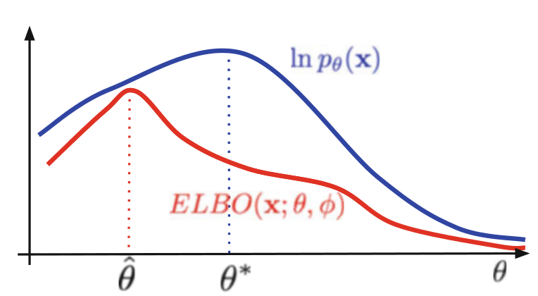
ELBO is lower bound on the log-likelihood. As a result, θ-hat maximizing the ELBO does not necessarily coincide with θ* that maximizing ln p(x). The looser the ELBO is, the more this can bias maximum likelihood estimates of the model parameters.
The relationship between the ELBO and $\log P(\boldsymbol{x})$ has led to using variational bound as a model selection criterion. The premise is that the bound is a good approximation of the marginal likelihood, which provides a basis for selecting a model.
The mean-field variational family
Currently we have talked about ELBO in detail, to recall, ELBO transforms inference problems, which are intractable, into optimization problem by approximating a variational density function $q(\boldsymbol{z})$ to posterior distribution $P(\boldsymbol{z} \vert \boldsymbol{x})$. Now its’ interesting to note that posterior may be complex distribution with more than one mode (multimodal), and in that case choosing for e.g. unimodal distriution from variational family may not help to approximate the posterior. And this becomes a problem that is prevalent with real world data.
As a solution we can have some members of variational family all trying collectively to fit closely to the posterior. Every member will be governed by distinct factors e.g. Gaussian distribution but with different mean and variances. But this is not going to be tractable due to multitude of dependency, so we assume latent variables to be independent. This is mean-field variational family.
A generic member of mean-field variational family is
$$ \begin{align} q(\boldsymbol{z}) = q(z_1, … , z_m) = q_{\phi_1}(z_1) \cdot q_{\phi_2}(z_2)…q_{\phi_m}(z_m) = \prod_{j=1}^{m} q_{\phi_{j}}(z_{j}) \label{eq:13}\tag{13} \end{align} $$
$q_{\phi_j}(z_j)$ is a member of some variational family, and in optimization these variational factors $q_{\phi_j}$ are choosen in such a manner to maximize the ELBO. These variational factors can be parameters of the distribution.
Now lets apply a recently learned concept to bayesian mixture of Gaussians just like we did it earlier.
Bayesian mixture of Gaussians
Conider again the bayesian mixture of Gaussians.
$$ \begin{align} q(\boldsymbol{z}) &= q(\boldsymbol{\mu}, \boldsymbol{c}) \cr &= q(\boldsymbol{\mu} \vert \boldsymbol{c})q(\boldsymbol{c}) \cr &= q(\boldsymbol{\mu})q(\boldsymbol{c}) \cr &= q(\mu_1, …, \mu_K) q(c_1, …, c_n) \cr &= \prod_{k=1}^{K} q(\mu_k) \prod_{i=1}^{n} q(c_i) \label{eq:14}\tag{14}\cr &= \prod_{k=1}^{K}q_{\phi_k}(\mu_k;m_k, s_{k}^{2})\prod_{i=1}^{n}q(c_i;\psi_i) \label{eq:15}\tag{15}\cr \end{align} $$
We have to perform optimisation over these variational factors in order to update their values so that they will be able to come close to the posterior distribution. $\mu_k$ is mean value we sampled from equation ($\ref{eq:2}$), and after updating the variational factors this will become $m_k$, same goes for $c_i$, $\psi_i$.
$q_{\phi_k}(\mu_k;m_k, s_{k}^{2})$ is a Gaussian distribution on the $k^{th}$ mixture components’ mean parameter; its’ mean $m_k$ and its’ variance is $s_{k}^{2}$. The factor $q(c_i;\psi_i)$ is a distribution on the $i^{th}$ observations’ mixture assignment which gives the probability of sampling $x_i$ from all the clusters in vector.
Mean-field family is expressive because it can capture any marginal density of the latent variables [1]. But every latent variable being independent loses the power of accounting correlations between them, making all the entries in the covariance matrix zero except the main diagonal. Such that, mean field doesn’t have only pros but cons too.
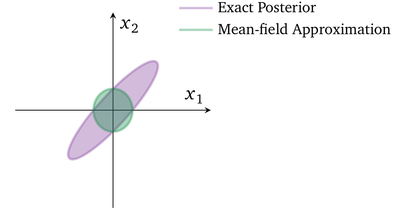
Visualization of mean-field approximation to a two-dimensional Gaussian posterior.
In the above figure, it is mean-field variational density after mazimizing the ELBO. This mean-field approximation has same mean as the original posterior density but the covariance structure is decoupled. KL-Divergence penalizes placing probability mass in $q(\cdot)$ on areas where $p(\cdot)$ has more mass, but less than it penalizes placing probability mass in $q(\cdot)$ on areas where $p(\cdot)$ has little mass. And that it has done in above figure, but in order to have successful match of densities, $q(\cdot)$ would have to expand into territory where $p(\cdot)$ has little mass.
Coordinate ascent mean-field variational inference
Till now we have talked about intractability of Bayesian mixture of Gaussians and to solve this we introduced ELBO, but just introducing ELBO wont’ help us since posterior distribution may be multimodal and to aid this approximation using our variational density we introduced mean-field variational family. But, our goal is still to maximize ELBO, and these stated concepts will help in that.
Coordinate ascent mean-field variational inference (CAVI) is commonly used algorithms for solving this optimization problem. CAVI iteratively optimizes each factor ($q_{\phi_i}$) of mean-field variational density, while holding others fixed(because of independency of latent variables). It climbs the ELBO to local optimum.
Using equation ($\ref{eq:10}$), we know $ ELBO(q(\boldsymbol{z})) = \mathbb{E_{z \sim q(\boldsymbol{z})}} \left [ \log \displaystyle \frac{P(\boldsymbol{x}, \boldsymbol{z})}{q(\boldsymbol{z})} \right ]$.
$$ \begin{align} \newcommand{\E}{\mathbb E} \E_{\boldsymbol{z} \ \sim \ q(\boldsymbol{z})}[\log q(\boldsymbol{z})] &= \E_{\boldsymbol{z} \ \sim \ q(\boldsymbol{z})}\Big[\sum_{j=1}^m \log q_{\phi_j}(z_j)\Big] \cr &= \sum_{j=1}^m \E_{z_j \ \sim \ q(z_j)}[\log q_{\phi_j}(z_j)] \cr &= \quad \E_{z_i \ \sim \ q_{\phi_i}(z_i)}[\log q_{\phi_i}(z_i)] \cr & \quad + \sum_{k \vert k \ne i} \E_{z_k \ \sim \ q_{\phi_k}(z_k)}[\log q_{\phi_k}(z_k)] \cr &= \quad \E_{z_i \ \sim \ q_{\phi_i}(z_i)}[\log q_{\phi_i}(z_i)] \cr & \quad + \ \ \overbrace{\E_{z_{-i} \ \sim \ q_{\phi_{-i}(z_{-i})}}[\log q_{\phi_{-i}(z_{-i})}]}^{ z_{-i} \text{ is fixed}} \cr &= \E_{z_i \ \sim \ q_{\phi_i}(z_i)}[\log q_{\phi_i}(z_i)] + \text{ const} \label{eq:16}\tag{16} \end{align} $$
$$ \begin{align} \newcommand{\E}{\mathbb E} \E_{\boldsymbol{z} \ \sim \ q(\boldsymbol{z})}[\log P(\boldsymbol{x, z})] &= \oint_{\boldsymbol{z}} q(\boldsymbol{z})\log P(\boldsymbol{x,z}) \ d\boldsymbol{z} \cr &= \int_{z_1}\dotsi\int_{z_m}\prod_{j=1}^mq_{\phi_j}(z_j)\log P( \boldsymbol{x, z}) \ dz_1 … \ dz_m \cr &= \int_{z_j}q_{\phi_j}(z_j)\int_{z_1}\dotsi\int_{z_{j-1}}\int_{z_{j+1}}\dotsi\int_{z_m} \prod_{k \vert k \ne j}q_{\phi_k}(z_k) \cr & \qquad \log P(\boldsymbol{x, z}) \ dz_1…dz_m \cr &= \int_{z_j}q_{\phi_j}(z_j)\Big[\oint_{z_{-j}}q(z_{-j})\log P(\boldsymbol{x, z})\ dz_{-j}\Big] \ dz_j \cr &= \int_{z_j} q_{\phi_j}(z_j)\E_{z_{-j} \ \sim \ q(z_{-j})}[\log P(\boldsymbol{x,z})] \ dz_j \cr &= \E_{z_j \ \sim \ q_{\phi_j}(z_j)}[\E_{z_{-j} \ \sim \ q(z_{-j})}[\log P(\boldsymbol{x, z})]] \label{eq:17}\tag{17}\cr \end{align} $$
Using equation ($\ref{eq:16}, \ref{eq:17}$), our ELBO($q(\boldsymbol{z})$) will be,
$$ \begin{align} \newcommand{\E}{\mathbb E} ELBO(q(\boldsymbol{z})) &= \quad \E_{z_j \ \sim \ q_{\phi_j}(z_j)}[\E_{z_{-j} \ \sim \ q_{\phi_{-j}}(z_{-j})}[\log P(\boldsymbol{x, z})]] \cr & \quad - \ \ \E_{z_j \ \sim \ q_{\phi_j}(z_j)}[\log q_{\phi_j}(z_j)] \ - \ \text{const} \cr &= \quad \E_{z_j}[\E_{z_{-j}}[\log P(\boldsymbol{x, z})] \ - \ \log q_{\phi_j}(z_j)]] \ - \ \text{const} \label{eq:18}\tag{18}\cr \end{align} $$
Coming back to our goal of doing all these calculations, we would like to maximize the value of ELBO. Now, to find the value for which a function gives maximum we do differentiation of that function an find stationary points or in simple words keep it equal to zero. Since we have decomposed the $q(\boldsymbol{z})$ into independent variational density functions,
we want
Now, while optimizing one of the variational density function $q_{\phi_j}$, we fixed the other variational factors/density functions $q_{\phi_{-j}}$, such that the optimization of former doesnt’ depend on latter in any case. Using this understanding we can independently optimize each variational factor.
$$
\begin{align}
q_{\phi_j}^{*} = \arg \max_{q_{\phi_j}} ELBO(q_{\phi_j}) \label{eq:20} \tag{20}
\end{align}
$$
Lets’ expand the ELBO($q(\boldsymbol{z})$), using equation ($\ref{eq:18}$)
Through optimization we would like to obtain optimal variational factor $q_{\phi_j}^{*}(z_j)$, but this function is itself dependent on $z_j$. For some $z_j$ we can have many different members of variational family giving maximum ELBO and that is why its’ functional or some researchers say function of a function. This cannot be optimized using regular derivative, but functional derivative.
We will not go into the depths of functional derivative in this blog. Although, Euler-Langrange equation can be used to solve this. This equation states that,
$$ \begin{align} \displaystyle \frac{\partial F}{\partial f} - \frac{d}{dx} \frac{\partial F}{\partial f’} = 0 \end{align} $$
where,
- $F$ is Functional and is equal to $q_{\phi_j}(z_j)[\mathbb{E_{z_{-j}\ \sim \ q_{\phi_{-j}}(z_{-j})}}[\log P(\boldsymbol{x}, \boldsymbol{z})] - \log q_{\phi_j}(z_j)]$
- $f$ is function that we want to optimize over, here its’ $q_{\phi_j}(z_j)$
- $f’$ is derivative of $f$
Note, $\displaystyle \frac{\partial F}{\partial f’} = 0$, since $F$ doesnt’ contain any term that has differentiation of $q_{\phi_j}(z_j)$. So, only $\displaystyle \frac{\partial F}{\partial f}$ is left and it will be equal to zero.
$$ \begin{align} \newcommand{\E}{\mathbb E} \displaystyle {\partial F \over \partial q_{\phi_j}(z_j)} &= \displaystyle {\partial \over \partial q_{\phi_j}(z_j)} \Big[q_{\phi_j}(z_j)[\E_{z_{-j}}[\log P(\boldsymbol{x,z})] \ - \ \log q_{\phi_j}(z_j)]\Big] \cr 0 &= \E_{z_{-j}}[\log P(\boldsymbol{x,z})] \ - \ \log q_{\phi_j}(z_j) \ - \ 1 \cr q_{\phi_j}^{*}(z_j) &= e^{\E_{z_{-j}}[\log P(\boldsymbol{x,z})] \ - \ 1} \cr &\propto e^{\E_{z_{-j}}[\log P(\boldsymbol{x,z})]} \label{eq:21}\tag{21} \end{align} $$
Lets’ have a look to a visualization regarding what all we have learned so far,
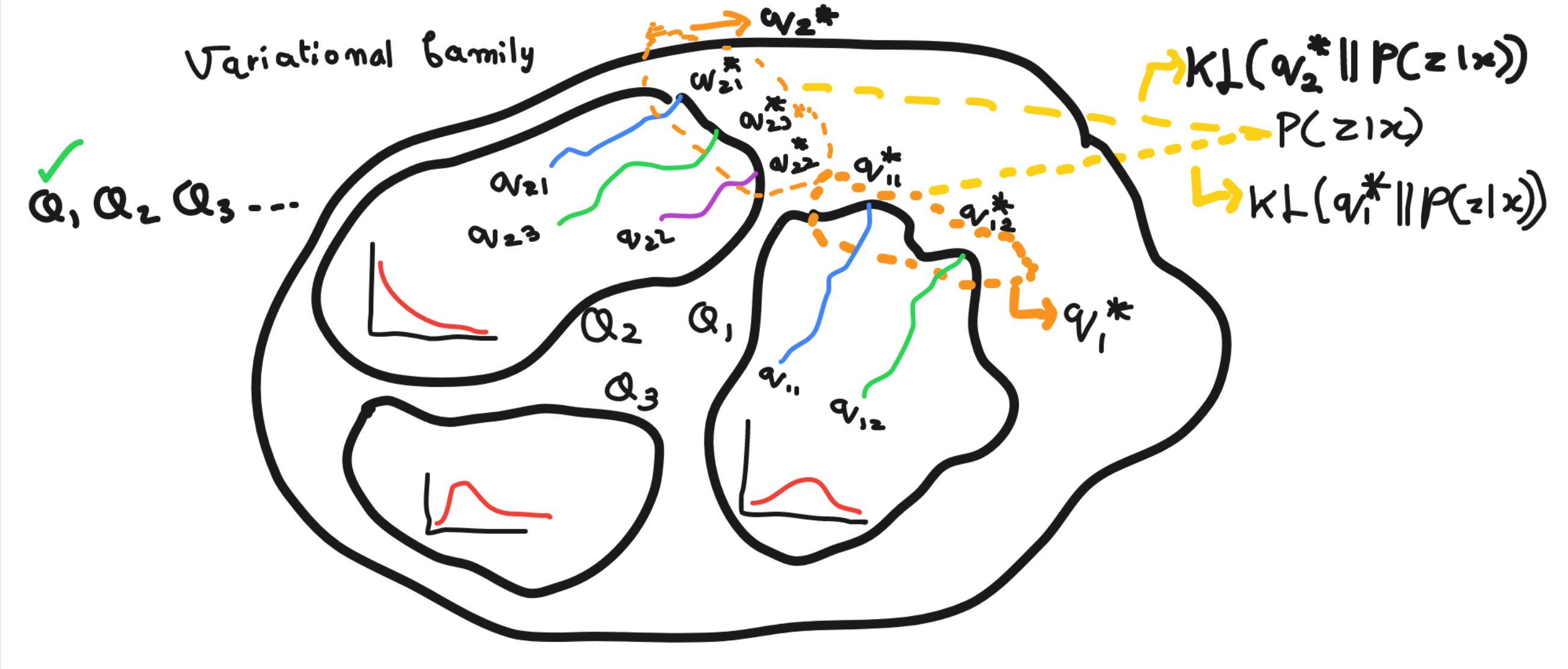
In this visualization we have variational family space consisting of three members of some density function. We choose randomly one family of three and then randomly initialized some clusters for e.g. K=2 in Q1, K=3 in Q2. Optimization than gave us variational parameters of these variational factors which closes up to posterior.
"""
Coordinate ascent variational inference (CAVI) Algorithm
"""

Input -> A model P(x, z), a dataset x
Output -> A variational density q(z) = q1(z1)...qm(zm)
Initialize -> Variational factors qj(zj)
while ELBO(t+1)-ELBO(t) >= δ:                 # converge
    for j in range(1, m+1):
       qj(zj) ∝ exp{E{-j} [log P(z, x)]}      # set
    ELBO(q) = E[log P(z, x)] - E[log q(z)]    # compute
return q(z)
Practicalities
Lets’ talk about few things to keep in mind while implementing and using variational inference in practice.
Initialization
The ELBO is (generally) a non-convex objective function and hence, there can exist exponential number of local optimums. CAVI only guarantees convergence to a local optimum, which can be sensitive to initialization.
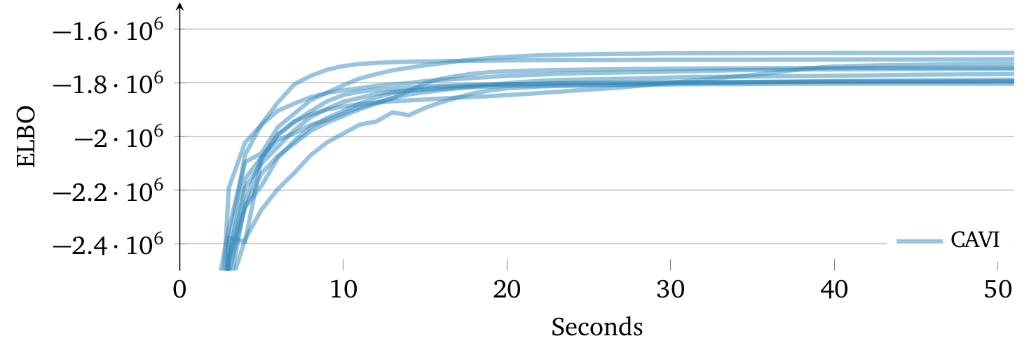
ELBO trajectory of 10 random initializations using Gaussian mixture model. Means of each variational factor is randomly sampled from another Gaussian distribution. Different initializations may lead CAVI to find different local optima of the ELBO
Assessing Convergence
We typically assess convergence once the change in ELBO has fallen below some small threshold. However, computing ELBO of the full dataset may be undesirable. Instead, its’ suggested to compute the average log predictive of a small held-out dataset.
Numerical Stability
Probabilities are constrained to live within [0, 1]. Precisely manipulating and performing arithmetic of small numbers require additional care. Thats’ why its’ recommended to work with logarithms of probabilities. One useful trick is log-sum-exp trick,
$$ \begin{align} \log \Big[\sum_i e^{x_i}\Big] &= \alpha + \log \Big[\sum_ie^{x_i-\alpha}\Big] \label{eq:22}\tag{22} \end{align} $$
where, $\alpha = \max\limits_i x_i$
A complete example: Bayesian mixture of Gaussians
In this section we are going to account the above concepts in order to set yet another example on bayesian mixture of Gaussians. So, we will first start notating the variables even though not much is going to change from what we notated in Bayesian mixture of Gaussians.
Consider $K$ mixture components and $n$ real-valued data points $x_{1:n}$. The latent variables are $K$ real-valued mean parameters $\boldsymbol{\mu} = \mu_{1:K}$ and $n$ latent-class assignments $\boldsymbol{c} = c_{1:n}$. Assignment $c_i$ indicates which latent cluster $x_i$ comes from. As usual, $c_i$ is $K$-vector indicator just like earlier. There is fixed hyperparameter $\sigma^2$, the variance of the normal prior on the $\mu_k$. We assume observation variance is $\boldsymbol{1}$.
Recall from equation ($\ref{eq:15}$), there are two type of variational parameters- categorical parameters $\psi_i$ for approximating posterior cluster assignment of the $i^{th}$ datapoint and Gaussian parameters $m_k$ and $s_{k}^{2}$ for approximating the posterior of the $k^{th}$ mixture component.
Lets’ find ELBO($q(\boldsymbol{m}, \boldsymbol{s^2}, \boldsymbol{\psi})$) by omitting latent variables.
$$ \newcommand{\E}{\mathbb E} \begin{align} \mathscr{L}(q(\boldsymbol{m, s^2, \psi})) &= \quad \E_{\boldsymbol{m, s^2, \psi} \ \sim \ q(\boldsymbol{m, s^2, \psi})} [\log P(\boldsymbol{x, m, s^2, \psi})] \cr & \quad - \ \ \E_{\boldsymbol{m, s^2, \psi} \ \sim \ q(\boldsymbol{m, s^2, \psi})} [\log q(\boldsymbol{m, s^2, \psi})] \cr &= \quad \E \Big[\log P(\boldsymbol{\mu; m, s^2})\Big] \cr & \quad + \ \ \E\Big[\log\prod_{i=1}^nP(c_i;\psi_i)P(x_i\vert c_i, \boldsymbol{\mu}; \psi_i, \boldsymbol{m, s^2})\Big] \tag{eq. 6}\cr & \quad- \ \ \E\Big[\log \prod_{k=1}^Kq_{\phi_k}(\mu_k;m_k, s_k^2)\prod_{i=1}^nq(c_i; \psi_i)\Big] \tag{eq. 15}\cr &= \quad \E[\log P(\boldsymbol{\mu; m, s^2})] + \sum_{i=1}^n\E[\log P(c_i; \psi_i)] \cr & \quad + \ \ \sum_{i=1}^n\E[\log P(x_i \vert c_i, \boldsymbol{\mu}; \psi_i, \boldsymbol{m, s^2})] \cr & \quad - \ \ \sum_{i=1}^n \E[\log q(c_i;\psi_i)] - \sum_{k=1}^K \E[\log q_{\phi_k}(\mu_k; m_k, s_k^2)] \label{eq:23}\tag{23}\cr \end{align} $$
Where, $\mathscr{L}$ is variational energy/ELBO (just different name and notations but same quantity). Using equations ($\ref{eq:6}, \ref{eq:15}$) we expanded the $\log$ quantities. We got equation () by combining the joint and mean-field family to form the ELBO for mixture of Gaussians, and it is function of variational parameters $\boldsymbol{m, s^2}$, and $\boldsymbol{\psi}$. Here, each expectation can be computed in closed form.
CAVI algorithm first derive the update for the variational cluster assignment factor $\boldsymbol{\psi}$; second, it derives the update for the variational component factor $\boldsymbol{\mu, s^2}$.
Variational density of mixture assignments
Before deriving the variational update for the cluster assignment $c_i$, lets’ do some preliminary calculations using equation ($\ref{eq:21}$).
we have on the right hand side,
$$ \begin{align} \newcommand{\E}{\mathbb E} \E_{z_{-j}} [\log P(\boldsymbol{x, z})] &= \E_{z_{-j} \ \sim \ q_{\phi_{-j}}(z_{-j})}[\log P(\boldsymbol{x} \vert \boldsymbol{z})P(\boldsymbol{z})] \cr &= \E_{z_{-j}}[\log P(\boldsymbol{x} \vert \boldsymbol{z})] + \overbrace{\E_{z_{-j}}[\log P(z_j)P(z_{-j})]}^{z_i \text{ is independent to } z_k, \ k \ne i} \cr &= \E_{z_{-j}}[\log P(\boldsymbol{x} \vert \boldsymbol{z})] + \overbrace{\log P(z_j)}^{\text{const wrt } z_{-j}} + \overbrace{\text{const}}^{z_{-j} \text{ is fixed}} \label{eq:24}\tag{24} \cr \implies q^{*}(z_j) &\propto e^{\E_{z_{-j}}[\log P(\boldsymbol{x} \vert \boldsymbol{z})] + \log P(z_j)} \label{eq:25}\tag{25} \end{align} $$
Using equation ($\ref{eq:25}$) we can derive the variational update for the cluster assignment $c_i$ like this,
$$ \newcommand{\E}{\mathbb E} \begin{align} q^{*}(c_i; \psi_i) \propto e^{\log P(c_i) + \overbrace{\E[\log P(x_i \vert c_i, \boldsymbol{\mu;m,s^2})]}^{\text{only } x_i \text{ corresponds to } _i}} \label{eq:26}\tag{26} \end{align} $$
In the above equation, we want to find variational update only for $c_i$, hence accounting $x_{-i}$ would not be essential. Assignment update may also depend on all the clusters’ variational parameters like mean and variance, so we accounting $\boldsymbol{\mu}$.
$\log P(c_i)$ is log prior of $c_i$ and is same for all possible values of $c_i$, $\log P(c_i) = -\log K$. Second term is the expected $\log$ of the $c_i^{th}$ Gaussian density. Since $c_i$ is indicator vector, we can write
$$ \begin{align} P(x_i \vert c_i, \boldsymbol{\mu}) = \prod_{k=1}^KP(x_i \vert \mu_k)^{c_{ik}} \label{eq:27}\tag{27} \end{align} $$
We can use this to compute the expected log probability,
$$ \begin{align} \newcommand{\E}{\mathbb E} \E_{c_i, \boldsymbol{\mu} \ \sim \ q(c_i, \boldsymbol{\mu})}[\log P(x_i \vert c_i, \boldsymbol{\mu})] &= \sum_{k=1}^K c_{ik} \E_{c_i, \boldsymbol{\mu} \ \sim \ q(c_i, \boldsymbol{\mu})}[\log P(x_i \vert \mu_k);m_k,s_k^2] \cr &= \sum_{k=1}^Kc_{ik}\E\Big[\log \frac{1}{\sqrt{2\pi}\sigma}e^{-\frac{(x_i-\mu_k)^2}{2\sigma}};m_k,s_k^2\Big] \cr &= \sum_{k=1}^Kc_{ik}\E\Big[\frac{(x_i-\mu_k^2)}{2};m_k,s_k^2\Big] + \text{const} \cr &= \quad \sum_{k=1}^Kc_{ik} \Big(\E[\mu_k;m_k,s_k^2]x_i-\E[\frac{\mu_k^2;m_k,s_k^2}{2}]\Big) \cr & \quad + \ \ \text{const} \label{eq:28}\tag{28}\cr \end{align} $$
Looking at equation ($\ref{eq:4}$) we can see that $P(x_i \vert \mu_k)$ corresponds to Gaussian distribution. Initially variance is set to 1, but during variational update it will be updated, right now we just need to know expression using which we can update. Equation ($\ref{eq:28}$) requires the calculation of $\mathbb{E}[\mu_k]$ and $\mathbb{E}[\mu_k^2]$ for each mixture component, both computable from variational Gaussian on the $k^{th}$ mixture component.
Thus the variational update for the $i^{th}$ cluster assignment is,
$$ \begin{align} \newcommand{\E}{\mathbb E} \displaystyle \psi_{ik} \propto \displaystyle e^{\displaystyle \E[\mu_k;m_k,s_k^2]x_i-\displaystyle \frac{\E[\mu_k^2;m_k,s_k^2]}{2}} \label{eq:29}\tag{29} \cr \end{align} $$
$\psi_{ik}$ is the probability that the $i^{th}$ observation comes from the $k^{th}$ cluster. So it is only a function of the variational parameters for the mixture of components.
We can also write a vectorized version of $\boldsymbol{\psi}$ in this way,
$$ \newcommand{\E}{\mathbb E} \begin{align} \boldsymbol{\psi} \propto \displaystyle e^{\displaystyle \boldsymbol{c}\Big(\boldsymbol{x}\E[\boldsymbol{\mu}; \boldsymbol{m, s^2}] - \frac{\E[\boldsymbol{\mu^2}; \boldsymbol{m, s^2}]}{2}\Big)} \end{align} $$
Variational density of the mixture-component means
Again using equation (\ref{eq:25}) we write down the joint density upto normalizing constant,
$$ \newcommand{\E}{\mathbb E} \begin{align} \displaystyle{q(\mu_k) \propto e^{\log P(\mu_k) + \overbrace{\sum_{i=1}^n\E[\log P(x_i \vert c_i, \boldsymbol{\mu}); \psi_i,m_{-k}, s_{-k}^2]}^{x_i \text{ can be sampled from any } \mu_k}}} \label{eq:30}\tag{30} \cr \end{align} $$
We now calculate the unnormalized $\log$(since, no normalization factor on RHS) of this coordinate-optimal $q(\mu_k)$. Also, $c_i$ is an indicator vector, so $\psi_{ik} = \E[c_{ik};\psi_i]$. Now,
$$ \newcommand{\E}{\mathbb E} \begin{align} \log q(\mu_k) &= \log P(\mu_k) + \sum_{i=1}^n\E_{\mu_{-k}}[\log P(x_i \vert c_i, \boldsymbol{\mu}); \psi_i, m_{-k}, s_{-k}^2] + \text{const} \cr &= \log P(\mu_k) + \sum_{i=1}^n \E_{\mu_{-k}} [c_{ik}\log P(x_i \vert \mu_k); \psi_i] + \text{const} \cr &= \log \frac{1}{\sqrt{2\pi}\sigma}e^{-\frac{(0-\mu_k)^2}{2\sigma^2}} + \sum_{i=1}^n \E[c_{ik};\psi_i] \log P(x_i \vert \mu_k) + \text{const} \cr &= -\frac{\mu_k^2}{2\sigma^2} + \sum_{i=1}^n \psi_{ik} \Big(-\frac{(x_i-\mu_k)^2}{2}\Big) + \text{const} \cr &= -\frac{\mu_k^2}{2\sigma^2} + \sum_{i=1}^n \Big[\psi_{ik}x_i\mu_k - \psi_{ik}x_i\frac{\mu_k^2}{2}\Big] + \text{const} \cr &= \Big(\sum_{i=1}^n \psi_{ik}x_i\Big)\mu_k - \Big( \frac{1}{2\sigma^2} + \sum_{i=1}^n\frac{\psi_{ik}}{2}\Big)\mu_k^2 + \text{const} \label{eq:31}\tag{31}\cr \end{align} $$
Lets’ not forget that our goal is still to maximize ELBO but by finding the variational update for $m_k, s_k^2, \psi_{ik}$. And for finding the value of these varational factors that will maximize ELBO(q($m_k, s_k^2, \psi_{ik}$)), we need to differentiate the above expression and keep it equal to 0.
Lets’ first take derivative with respect to $\mu_k$.
$$ \begin{align} \frac{\partial }{\partial \mu_k} \log q(\mu_k) &= 0 \cr \Big(\sum_{i=1}^n \psi_{ik}x_i\Big) - \Big( \frac{1}{\sigma^2} + \sum_{i=1}^n\psi_{ik}\Big)\mu_k &= 0 \cr \mu_k = m_k &= \boxed{{\sum_{i=1}^n \psi_{ik}x_i \over {\frac{1}{\sigma^2} + \sum_{i=1}^n\psi_{ik}}}} \label{eq:32}\tag{32}\cr \end{align} $$
Similarly for $s_k^2$,
$$ \begin{align} s_k^2 = \boxed{\frac{1}{\frac{1}{\sigma^2} + \sum_{i=1}^n\psi_{ik}}} \label{eq:33}\tag{33} \end{align} $$
The coordinate optimal variational density of $\mu_k$ belongs to exponential family of distribution, where sufficient statistics ${ \mu_k, \mu_k^2 }$ and natural parameters ${ \sum_{i=1}^n \psi_{ik}x_i, -\frac{1}{2\sigma^2}-\sum_{i=1}^n \frac{\psi_{ik}}{2} }$. This shows its’ a Gaussian distribution.
"""
CAVI for a Gaussian mixture model
"""

Input -> x(1:n), K, prior variance σ^2
Output -> q(µ_k; m_k, s_k^2) (Gaussian) and q(c_i; ψ_i) (K-categorical)
Initialize -> m(1:K), s^2(1:K), ψ_i(1:n)

while ELBO(t+1)-ELBO(t) >= δ:               # converge
   for i in range(1, n+1):
      ψ_ik ∝ exp{E[µ_k; m_k, s_k^2]x_i
               - E[µ_k^2; m_k, s_k^2]/2}    # set
   for k in range(1, K+1):
      m_k   <- equation 32                  # set
      s_k^2 <- equation 33                  # set
   ELBO[m, s^2, ψ]                          # compute
return q(m, s^2, ψ)
Great, now lets’ talk about some benefits along with limitations of Variational Inference.
Benefits
- Faster to converge than MCMC and easier to scale to large data
- Applied to real world problems like :-
- Large-scale doument analysis
- Computational Neuroscience
- Computer Vision
- Because its’ optimization problem, usage of stochastic optimization along with comes handy
- Doesnt’ suffer in accuracy, i.e. in terms of posterior predictive densities
This is why, variational inference is suitable for problems that contain large datasets and we want to quickly explore many models. For e.g. fitting a probabilistic model of image to millions or billions of images.
Limitations
- Studied less rigorously than MCMC due to which we havent’ been able to uleash its’ full potential
- It doesnt’ provide asymptotic guarantees of convergence, but only find density close to target
Conclusion
We started with defining and understanding the core problem in bayesian statistics or regarding predictive analysis in general. From there we found two approaches to solve this problem, one is Monte Carlo Markov Chain (MCMC) technique regarding whih we had brief discussion and another is Varational Inference which is the center of attraction for this article. MCMC method has been in use since before variational inference was even introduced, so we talked about about the shortcomings of former for th introduction of latter. Now, from ground-up we talked about variational inference using derivations and examples from mixture of Gaussians. Variational Inference is definitely a path forward that we can see by the ubiquity of machine learning methods like VAEs.
$$\color{#A91B0D}\text{Thankyou for your time and patience}$$
Citation
Cited as:
Garg, P. (2023, May 11). Autoregressive Models: Connecting the Dots. Eulogs. Retrieved May 11, 2023, from https://www.eulogs.com/posts/variational-inference-the-path-forward/
or
|
|
References
[1] Blei, D. M., Kucukelbir, A., & McAuliffe, J. (2016). Variational Inference: A Review for Statisticians. Journal of the American Statistical Association, 112(518), 859–877. https://doi.org/10.1080/01621459.2017.1285773
[2] Van Ravenzwaaij, D., Cassey, P., & Brown, S. D. (2018). A simple introduction to Markov Chain Monte–Carlo sampling. Psychonomic Bulletin & Review, 25(1), 143–154. https://doi.org/10.3758/s13423-016-1015-8
[3] Tomczak, J. M. (2022). Deep Generative Modeling. Springer Nature